I got two parking tickets, so I trained a VLM

In April I drove up from San Jose and spent a week in San Francisco. I came back with good memories and two parking tickets. Both for the same reason: I stood in front of a pole holding four signs, read all four, and still could not work out whether I was allowed to leave my car there.

You know the pole. A 2-hour limit. Except with an Area S permit. Except it is also a street-cleaning zone on Tuesday mornings. Also tow-away during evening rush. Each sign is perfectly legible on its own. Stacked together they form a little logic puzzle with a time variable, and my brain, mid-errand and already late, refused to solve it. Twice. That is about $160 of tuition.

The maddening part is that every fact you need is printed right there on the metal. It is pure perception, plus rule-logic, plus a clock. Which is a very machine-shaped problem. So I asked the obvious question:

Can a small, cheap, runs-on-a-phone vision-language model do the thing my brain failed to do?

The off-the-shelf one cannot. But you can teach it. I called the project curbcheck, and this is how it went.

The trap is the stack, not the sign

A single sign is easy. Modern VLMs read “2 HOUR PARKING 9AM TO 6PM” without breaking a sweat. The difficulty is combinatorial: the moment you stack three or four restrictions on one pole, the model has to read all of them correctly and combine them under a specific day and time. Miss one faded sign at the bottom and the whole verdict flips from “fine” to “your car is on a flatbed.”

So the interesting unit is never one sign. It is the pole.

Read, then reason

The lazy design is to show the model a photo and ask “can I park here?” and trust whatever sentence comes out. I did not want that, for two reasons. First, an end-to-end verdict hides its mistakes inside confident prose. Second, I wanted to actually learn the signs myself, not outsource my brain forever.

So curbcheck splits the job in two:

photo  ->  VLM reads each sign to JSON  ->  deterministic resolver  ->  verdict + reason

The vision-language model only does perception. It reads the pole into structured rules: kind, days, hours, time limits, permit area, even “2nd and 4th Tuesday of the month.” Then a tiny deterministic resolver (plain Python, no model in the loop) takes those rules plus the current time and returns the verdict. Both halves are shown to you, so a misread is visible instead of buried.

That split turns out to be the whole ballgame. The resolver never fumbles the logic, no matter how many signs are on the pole. All the difficulty collapses onto one question: did the model read the pole correctly?

Making data out of thin air

There is no dataset of “SF parking poles with ground-truth rules.” So I made one.

The synthetic half is a renderer that draws CA-style sign plates from public Caltrans sign specs (the R26 no-parking, R30 time-limit, and R32 street-cleaning families), stacks one to four of them on a pole, and ships every pixel with exact ground truth, because I generated the rules first and drew them second. To keep the rule distributions realistic rather than uniform-random, I seeded them from SFMTA’s public inventory of 144,333 actual street signs.

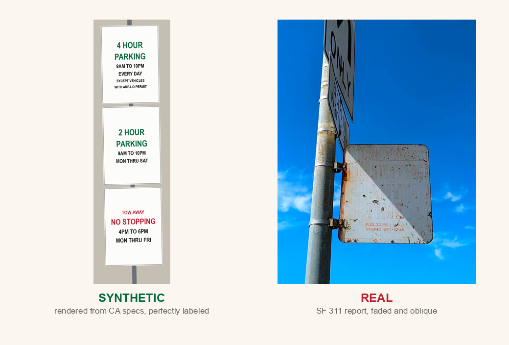Left: a clean synthetic render. Right: the real world, where signs are faded, tilted, sticker-covered, and shot from a moving car. The gap between these two is the entire story of this project.

The real half came from SF’s open data: DPW street-space permit photos and 311 reports, which are full of close-up sign photos. I had a frontier model (Claude Opus) label them as a teacher, then verified a chunk by hand. The final mix is roughly 77% synthetic, 23% real.

The student

The model is Qwen2.5-VL-3B, fine-tuned with QLoRA (rank 16) on the language layers only, with the vision encoder frozen, trained on a rented A100. Small, cheap, and the kind of thing that could plausibly run on a phone someday. Remember that frozen vision encoder. It comes back to bite me later.

Does it work?

On the synthetic benchmark, embarrassingly well.

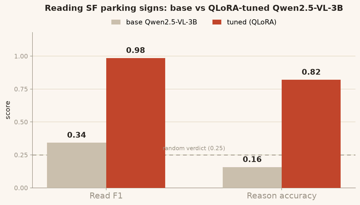Read F1 and reasoning accuracy, base Qwen2.5-VL-3B versus the QLoRA-tuned version.

A stock Qwen2.5-VL-3B scores 0.16 on “can I park here right now,” which is below the 0.25 you would get by guessing among four verdicts at random. One QLoRA run takes it to 0.82 reasoning and 0.98 read accuracy.

And it scales exactly the way the parking-ticket story predicts, with the number of signs on the pole:

Signs on the pole	Tuned reasoning accuracy
1 sign	0.95
2 signs	0.80
3 signs	0.67
4 signs	0.56

That last row is the exact pole that cost me two tickets. The model is now meaningfully better at it than I was.

The honest part

Here is where I have to be a grown-up about it. Synthetic numbers are easy to fall in love with, and the real world is where projects go to be humbled.

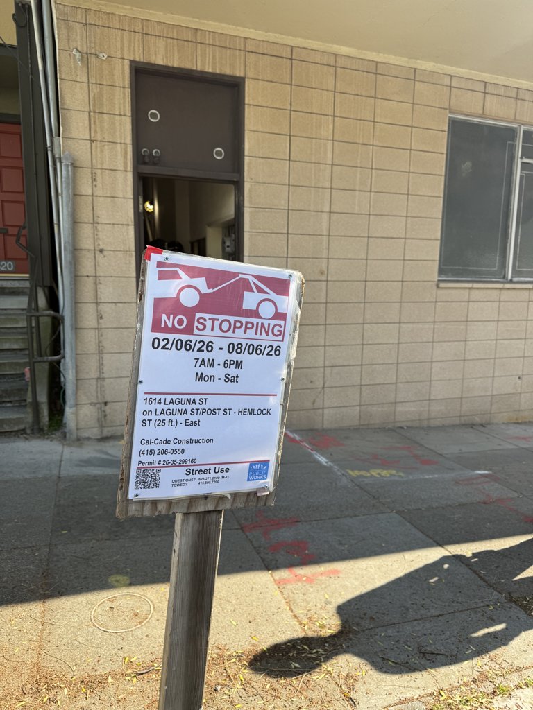A real pole from the test set. Faded, oblique, shot outdoors. Much harder than a clean render.

On held-out real SF photos, reading is genuinely hard:

Metric (real photos)	base	tuned
Read F1	0.04	0.34
Pipeline reasoning	0.78	0.89

Two things jump out. The good: the deterministic resolver keeps pipeline reasoning at 0.89 even when reading is stuck at 0.34, which is exactly the payoff of the read-then-reason split. Partial reads still resolve correctly more often than not.

The humbling: I threw everything at the reading gap. I doubled the real training data, added human-verified labels, and augmented the renderer with fading, occlusion, and perspective. Real-photo reading moved from 0.33 to 0.34. One point.

That non-result is actually the most useful thing I learned. If more data barely moves the needle, the bottleneck is not data, it is model capacity. And the prime suspect is that frozen vision encoder I mentioned earlier. The model can reason about signs it reads; it just cannot reliably read faded, sun-bleached Mission Street poles with a vision tower that never got to adapt. So the next experiment is not more data. It is unfreezing the vision encoder.

I ran the experiment. The hypothesis was wrong.

So I did it. I unfroze the vision encoder, roughly doubled the real training data by pulling parking-sign photos from other cities (Oakland, Chicago, and more), and replaced the single-pass labels with a 3-vote consensus.

Then I tested it the same way I tested everything else: on the full held-out set, no cherry-picking. The result was not what I predicted, and that was the interesting part.

Metric (real photos)	base	first tune	vision unfrozen + more data
Read F1	0.04	0.34	0.33
Reasoning (pipeline)	0.78	0.89	0.90
Reasoning (end to end)	0.09	0.41	0.82

Reading did not move. 0.34 to 0.33. Unfreezing the vision encoder, the thing I was sure was the bottleneck, did nothing for it. So that hypothesis was wrong too.

But look at the bottom row. End-to-end reasoning on real photos doubled, 0.41 to 0.82. The diverse cross-city data and cleaner labels did not teach the model to read better; they taught it to reason better about what it does read, and to stop over-calling restrictions on simple poles.

I had one idea left for reading: bolt on a small dedicated OCR model, plus a contrast-normalization transform to rescue faded signs. On a handful of hard images I picked by hand, it looked promising. So I ran a proper A/B across the entire test set before believing it.

It made things worse. OCR text as a hint confused the model on the clean signs it already read fine, and the contrast trick recovered nothing on average. A clean reminder of why you test on the whole set, not the three examples that flatter your idea.

So here is the honest state. Reading faded, cluttered SF sign poles is genuinely hard, and not because of one fixable bottleneck. The model reads simple 1-to-2-sign poles decently and falls apart on dense 4-sign ones. What carries the product is the architecture: because a deterministic resolver does the logic, the verdict stays right about 90% of the time even when a read is imperfect. The neural net is allowed to be the fallible part.

Update: the reading number was a measurement bug

After all that hand-wringing about reading being stuck at 0.33, I found the real culprit, and it was my own scorer.

Half the eval set (231 of 500 photos) is downed or missing poles with no readable sign. The correct answer there is to read nothing, an empty list. My read-F1 scorer was counting that correct “nothing” as a zero instead of a perfect score. So nearly half the benchmark was punishing the model for correctly abstaining.

Once I fixed it, the real numbers are very different:

metric (real photos)	base	v5
Read F1, sign-bearing photos	0.08	0.62
Abstains correctly on no-sign photos	0.57	0.83

So the model reads real sign-bearing photos at about 0.62 F1 (around 0.52 against a stricter 3-vote consensus gold I built to de-noise the metric), and correctly says “no sign here” 83% of the time. Reading was never the 0.33 disaster I thought. It is decent on 1-to-2-sign poles and weakest on cluttered 4-sign ones.

The lesson, again: check the ruler before you trust the number. I built the consensus gold to ask whether the model was worse than the metric claimed. The answer turned out to be the opposite. The metric was worse than the model.

Scaling up: a 7B student, and a bug hiding in plain sight

The diagnostics kept pointing at one thing: reading real signs was capacity-bound, not data-bound. So I did the obvious next experiment and swapped the 3B student for a 7B one, trained on the full cross-city corpus (now 17 cities, cleaned with 3-vote consensus labels). Same read-then-reason architecture, just a bigger brain doing the perception.

On simple poles it clearly helped. The 7B reads a clean single-sign pole perfectly, and on real sign-bearing photos it edged the 3B up from about 0.62 to roughly 0.72 (on a smaller hand-checked sample). The pipeline verdict held around 0.92. The bigger model perceives more, exactly as the read-ceiling story predicted.

But the more interesting result came from splitting the score by how many signs are on the pole, instead of trusting one average. The moment I bucketed it, the aggregate number fell apart:

signs on the pole	7B read F1
1 sign	1.00 (perfect)
2 signs	partial
3 to 4 signs	~0.00

That “0.00” on dense poles looked catastrophic. It wasn’t. Digging into the raw outputs, the 7B was reading those poles and then never stopping. It emits the JSON and just keeps generating instead of producing an end-of-sequence token. So every dense-pole read ran to the length limit: truncated into invalid JSON when I capped tokens low, and painfully slow (tens of seconds each) when I capped them high. The 3B never did this. The 7B regressed on knowing when to shut up.

So the honest state of v6: bigger reads simple poles better, but it has a generation-termination bug on cluttered poles that a smaller, dumber model didn’t have. The fix is boring (constrain the stop token, or a short fine-tune that teaches clean endings). The lesson is not: a single averaged metric hid both a scoring mistake of mine and a real regression in the model. Bucket your eval before you believe it. The pole that beat me is still where the interesting failures live.

Update: the bug was boring, the audit was not

The termination bug turned out to be exactly as boring as predicted. Instead of retraining the model to say “I’m done,” I made the eval harness stop listening: a small stopping rule that ends generation the instant the JSON closes. Dense-pole reads went from fifty seconds to a few, and for the first time the full 500-photo real eval ran end to end with zero skipped samples. The “0.00 on dense poles” vanished the way artifacts do: the 7B actually reads synthetic 3-and-4-sign stacks essentially perfectly (0.99 overall).

With the full run finally measurable, the 7B’s real number came in at 0.735 F1 on sign-bearing poles. Better than the 3B’s 0.62. But the biggest remaining error pool was strange: 45 single-sign photos, the easy case, scored exactly zero. Simple poles the model supposedly could not read at all.

So I audited every one of them by hand (well, by agent: three vision models re-read each photo and adjudicated). The blame table was not what the metric claimed:

who was actually wrong	count
the model	14
the teacher’s gold labels	12
nobody (two valid names for the same sign)	7
the sign itself (graffiti, crop, too far away)	12

Only a third of my “model failures” were the model. The Opus teacher had encoded “12 NOON TO 2PM” as midnight-to-2am, labeled a Monday sign as Wednesday, and left times blank on signs where the times are perfectly legible. Set-wide, one in eight gold labels was malformed. I had been grading the student with the teacher’s mistakes.

The audit also flushed out something worse: a genuine logic bug in the deterministic resolver, the half of the system I had been bragging “is never wrong.” A pole whose only sign reads “TOW-AWAY, NO PARKING ANY TIME” fell through every branch of the verdict logic and came back as you can park here. At a tow-away zone. The eval had even baked that in as the correct answer, so no metric could ever catch it. It is fixed now, with regression tests, and it permanently upgraded my respect for the phrase “deterministic just means deterministically wrong.”

After fixing the labels, the naming coin-flips, and the resolver, the honest current scorecard:

metric (real photos)	v5 (3B)	v6 (7B)
Read F1, sign-bearing poles	0.62	0.83
Read F1, single-sign poles		0.88
Pipeline reasoning	0.90	0.89

Roughly 40% of what I had been calling a model gap was measurement. The general lesson stacks neatly on the earlier one: first I learned to check the ruler, then I learned the ruler’s labels need checking too. When a metric plateaus, do not buy more data or more GPU. Print the errors and read them with your own eyes. It is the cheapest experiment in machine learning and consistently the most embarrassing.

Try it

I wrapped the tuned model in a little demo. Upload a photo of an SF sign pole, pick a day and time, and it shows you both what each sign says and whether you can park. Try it right here:

Give it a few seconds to wake up, it runs on free ZeroGPU and naps when idle. If it’s asleep, the full Space is here.

• Demo: the curbcheck Space
• Model (the v5 adapter): shubhamgoel27/curbcheck-qwen25vl3b-v5-lora
• Code, benchmark, and the full, honest results: github.com/shubhamgoel27/curbcheck

It is not solved. Real-world reading is still the open problem, and I find that more interesting than if it had worked on the first try. But there is now a small model that gets the pole that beat me, and a clean experiment pointing at what to try next.

Still a little mad about those tickets. But at least they were tax-deductible as research.